Cat Detection from Scratch
Audience: Technically-minded readers who are curious about deep learning.
Reading time: ~22 minutes.
TL;DR. In 2017 I tried to train a neural network from scratch to detect cats and ended up with a digit classifier instead. The article walks the whole loop: the code, the long stream of training-progress numbers scrolling past on the terminal as the model learns, the knobs I turned in sequence (longer training, better optimizer, deeper architecture, regularization), and the wall I hit when I tried to point the same techniques at cats.
If you want only the feel of training from scratch and not the full walkthrough, skim past the prose and look at the green-tinted terminal blocks (marked “2017” in the upper right). Each is verbatim output from a real 2017 training run I did on an Nvidia V100. The shape of the numbers (noisy, bouncing, slowly climbing, sometimes locking at 100%) is most of what training feels like from the inside. One characteristic example, from the simplest model I trained:
step 0, training accuracy 0.12
step 1000, training accuracy 0.89
step 2000, training accuracy 0.87
step 3000, training accuracy 0.89
step 4000, training accuracy 0.85
step 5000, training accuracy 0.95
step 6000, training accuracy 0.86
step 7000, training accuracy 0.93
step 8000, training accuracy 0.9
step 9000, training accuracy 0.92
0.9158
10,000 steps of stochastic gradient descent on a single matrix multiplication. Training accuracy bouncing in the high 80s and low 90s, test accuracy of 91.58% on held-out digits. The rest of the article is what changes when you turn each knob, why the numbers do what they do, and what the loop is actually doing underneath the abstractions you already use. When I was done with this experiment, we got to a final accuracy of 99.35%.
In May 2017 I sat down to train a neural network from scratch. This was a learning project, and I started with cats as is traditional in computer vision, but the point was less the classifier itself and more the hands-on experience with deep learning that I had been missing. The actual product, as you will see, ended up being something different anyway.
I had been writing software for twenty-five years at that point, and managing ML teams since before AlexNet. An early-2010s team I led built real computer-vision systems on classical methods like random decision forests and hand-engineered features, the kind of pipeline that AlexNet would later vaporize. I had familiarity with ML techniques, but what I hadn’t done was train one of these networks myself, and by 2017 that felt like a gap worth closing. I knew Linux and Python, and had a working sense of linear algebra and a fading memory of multivariable calculus.
The plan was MNIST first, then cats. MNIST looks like this:
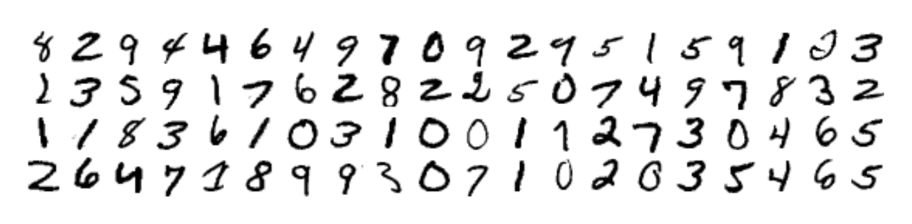
It is the “hello world” of computer vision, the way a Fibonacci function is the hello world of recursion. The plan was to use it as a warm-up before pointing the same techniques at full-color photographs of cats. What I trained instead was a digit classifier, and then a series of progressively better versions of it, and each step taught me something about training that I could not have learned by reading.
A footnote before we begin: a year or so after I wrote the original version of this study guide, I shared it with a recent University of Washington CS grad who was on my team. He told me it was basically the material from his first-year ML class. I am still not sure whether that was meant to sound critical. Either way, I was happy: landing at “first-year ML curriculum” felt like a reasonable destination for a self-directed side project, and it is roughly the altitude I am aiming to explore here.
Code blocks, terminal output, and indented quoted passages below are reproduced from the original 2017 study guide. The prose around them is from today, looking back. I use past tense for what actually happened in 2017 on the V100, and present tense for how the code or the math works in any era.
Training vs. inference
The first thing worth getting straight is that training and inference are two completely different workloads that happen to share a model file.
Inference is what you do every time you call a model: a forward pass through the network’s fixed weights, input in, prediction out. It is, computationally, a sequence of matrix multiplies. The weights are read-only. The cost is bounded and predictable.
Training is the part where those weights stop being a model and become a search problem. You start with random numbers in every weight matrix. You show the network an example, see how wrong its answer is, compute how each weight contributed to the wrongness, and nudge every weight in the direction that would have made the answer slightly less wrong. Then you do that several billion times.
This is the thing that’s hidden when you fine-tune through somebody else’s framework. The framework hands you a Trainer object that wraps a forward, a backward, an optimizer step, and a learning rate schedule. The actual mechanics (what the loss looks like as a scalar, how a gradient propagates back through a softmax, what an Adam optimizer is actually doing to your weight tensors) are usually a few abstraction layers down. If you have only ever seen training from above, you’ve seen the dashboard but not the engine.
So: cats. Or, as it turned out, digits.
Deep neural networks
It is worth sketching what “deep learning” actually is before we get into the code, because the audience for this post may have used these systems without ever working out how ML, deep learning, and LLMs relate.
Machine learning is the broad family of algorithms that learn patterns from data instead of being explicitly programmed. Classical ML included things like linear regression, decision trees, support vector machines, and a long tail of statistical methods. These worked well within their respective niches but plateaued through the 2000s on hard perceptual tasks like image, speech, and language understanding.
Deep learning is the particular flavor of ML that uses neural networks with many layers, trained end-to-end by gradient descent on a loss function. The ideas go back decades, but as a practical revolution it begins in 2012 with the AlexNet paper from Geoffrey Hinton’s group at Toronto, which won the ImageNet competition by a margin so wide it essentially obsoleted the previous generation of computer vision overnight. (Hinton would later share the 2024 Nobel Prize in Physics for foundational work on neural networks.) The combination that made AlexNet work was deeper networks than anyone had been training, GPUs fast enough to train them at that depth, and enough labeled data to feed them. Within a few years, deep learning had displaced classical methods in vision and speech, in machine translation, and across most other domains where signal had previously been wrung out of hand-crafted features. Each domain saw large step changes (ImageNet top-5 error fell from ~26% in 2011 to under 5% by 2015) and by 2012 it was clear the approach had years of further gains ahead of it.
Modern large language models are a form of deep learning. The 2017 “Attention is All You Need” paper introduced the transformer architecture, and scaling transformers massively on internet-scale text produced today’s LLMs. They are not a different paradigm. They are deep neural networks trained on a self-supervised objective (predicting the next token) using the same gradient descent, the same backpropagation, and the same family of operations (matrix multiplications and nonlinearities, stacked into deep architectures) as the small classifier I am about to walk you through. The transformer’s attention mechanism is itself “just” a particular composition of matrix multiplies. LLMs add components the simple CNN below does not have (attention, layer normalization, residual connections, positional encodings) and train on a vastly larger budget, but the conceptual machinery of “compute gradients, nudge weights, repeat” is shared. Understand the small case and you have most of the scaffolding for the large case.
A neural network is, structurally, a stack of layers. Each layer takes a vector of numbers (the activations of the previous layer), multiplies it by a matrix of learnable weights, adds a bias vector, and runs the result through a nonlinearity (a simple element-wise function like ReLU; without it, stacking layers gains nothing, since the whole stack collapses to one linear map). The output of one layer becomes the input of the next. The first layer sees your raw data; the last layer produces the answer. Everything in between is called a hidden layer, because nothing outside the network ever observes it directly.
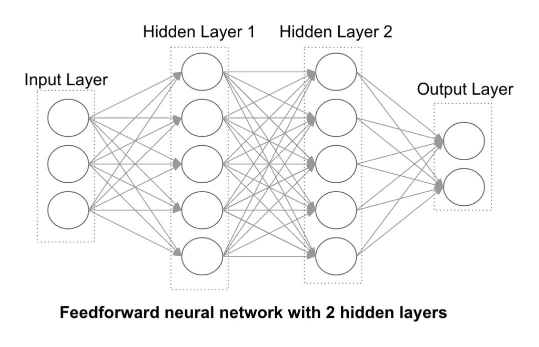
If you watch one excellent visual intro to ML and deep learning, watch 3Blue1Brown’s “But what is a neural network?” It animates a small MNIST classifier like we describe above.
More layers usually help. Stacking more hidden layers and training the whole stack end-to-end lets the network discover its own feature representations without you handcrafting them. Pre-2012, computer vision practitioners wrote code that extracted edges, corners, color histograms, and SIFT descriptors, and fed those features into a classifier. Post-2012, after AlexNet won the ImageNet competition, you fed raw pixels in and the network figured out the features for you. That shift, from human-designed features to learned representations, is what every “deep learning revolution” headline was actually about.
One piece of training discipline that matters across all of these architectures, and is worth flagging now since we’re about to use it: you do not train on all your data. You split it. The standard pattern is some variation of three buckets: a training set the model actually learns from, a validation set you use during training to tune hyperparameters and decide when to stop, and a held-out test set you only look at once, at the very end, to honestly estimate how the model will do in the wild. Exact ratios vary (80/10/10 and 60/20/20 are both common, and many production datasets use fixed splits or k-fold cross-validation instead).
The key invariant is the held-out test set. The reason for any of this is overfitting. It is trivially easy to produce a model that memorizes its training data perfectly and then collapses completely on anything it has not seen before. You will not know this is happening unless you have data the model was never allowed to look at during training. The test set is the only honest measurement you have. If you peek at it, tune against it, or train on it, you have given yourself nothing but vibes.
Why I didn’t just download a cat detector
Here is something a 2026 reader will find absurd: in 2017, “just download a state-of-the-art image classifier” was not a real option in the way it is now. ResNet existed (the paper had landed at the end of 2015), but I didn’t know about it. ImageNet existed. The pre-trained-model ecosystem existed, in the sense that the weights were out there, but the surrounding ergonomics had not arrived yet. There was no Hugging Face Hub. There was no from transformers import pipeline. There was a TensorFlow blog post or two with TODO-shaped instructions.
I didn’t know any of this. What I knew was that Andrew Ng, a Stanford ML professor and co-founder of both Coursera and Google Brain, had a series of excellent YouTube videos and that TensorFlow had a Python API. So I picked the well-trodden warm-up path: MNIST first, as shown above, with cats deferred to later. The expectation, in retrospect largely wrong, was that cats were going to be only a little harder than digits.
The setup in 2017
The GPU was an Nvidia V100 sitting in an AWS p3.xlarge EC2 instance. To set the scene, here is what I wrote in the original study guide a few months earlier, with all the wide-eyed enthusiasm of someone who had just discovered that you could rent serious compute by the hour:
For just a few dollars an hour, you can now access computational power equal to some of the world’s top supercomputers in 2006. Amazon Web Services (AWS) claims 70 teraflops (trillion floating point operations per second) on a single p2.16xlarge instance which includes 16 GPU cores, 64 vCPUs, and 732 GB RAM. And you can scale that out into a low-latency compute grid if you need more. Note that TensorFlow doesn’t automatically parallelize your model; you’ll need to specifically design your model to take advantage of more than one GPU.
That quote is about the p2 generation, with 16 Tesla K80s in the largest variant. By the second half of 2017, AWS had launched the new p3 instances with the much faster Nvidia V100 inside, and I had upgraded. The p3.xlarge was AWS’s flagship single-GPU instance, just over three dollars an hour, and getting access was not automatic. You had to submit a support request explaining what you were doing with the GPU, and the account had to be individually vetted before AWS would let you spin one up. I remember the small thrill of getting approved as the first time a cloud provider had treated me like I was being trusted with something serious. The V100 was the most powerful GPU you could rent on demand anywhere, and for three dollars an hour I could borrow one for an evening. In late 2017 that still felt a little like science fiction.
In 2026 the V100’s role as “the flagship single-GPU you rent for serious work” is played by the Nvidia H100, on the Hopper architecture, the direct data-center successor in NVIDIA’s lineage. An H100 instance on AWS runs around five dollars an hour, somewhat more than the V100 cost me in 2017, and is roughly five times faster on mixed-precision training workloads. No vetting required, no support ticket. The next generation (Blackwell) is already starting to show up in the same dropdown. The “powerful instance” bar has moved several rungs up the ladder, and the experience of using one has gone from “submit a support ticket and wait” to “pick it from a menu and click launch.” The deeper version of the same shift is that the felt-impossible-now-trivial machine of 2026 is the consumer Mac with enough RAM to run a 70B-parameter language model locally. The “wait, we can just do this?” feeling never really goes away, it just changes scope.
There was a pre-baked “Deep Learning AMI” image you could launch and get TensorFlow, CUDA, and Jupyter pre-installed, which was important because installing the right CUDA toolkit against a fresh Ubuntu from scratch was an exercise in spiritual development.
The framework was TensorFlow 1.x. In 2017 that felt like the obvious choice: TensorFlow was Google’s framework, it had Google’s full marketing weight behind it, and as far as I knew it was simply the deep learning framework. PyTorch had been released by Facebook the previous year and was working its way through the research community, but I had not yet seen it. With the benefit of hindsight, the bet I should have made was the other one. In the years since, PyTorch has become the framework I see most often when I look at what the top AI researchers and labs I have come to know actually reach for. TensorFlow is still excellent, still widely used, and still the right answer for plenty of production deployments. The choice between them is more like picking a programming language than picking sides. I am calling this out for any reader new to the space: the two main ecosystems for this kind of work are TensorFlow and PyTorch, they are largely interchangeable for the purposes of this post, and the code below being TensorFlow is an accident of 2017 timing rather than a recommendation.
TensorFlow 1.x specifically used a “build a graph, then run a session” model that has since been ripped out of TensorFlow itself and replaced with the eager execution model PyTorch had been doing all along. Every line of code in this post is from that era. I’m leaving it in TensorFlow 1.x because that is what the journey actually looked like, and because the shape of the loop is the same regardless of which framework you’d use today.
The smallest interesting training loop
Here is the first thing I trained. The whole program is about forty lines.
## mnist1.py

import tensorflow as tf

# download MNIST data from yann.lecun.com/exdb/mnist/
from tensorflow.examples.tutorials.mnist import input_data
mnist = input_data.read_data_sets("MNIST_data/", one_hot=True)

# create placeholder for 28x28 images
x = tf.placeholder(tf.float32, [None, 784])

# Weight & bias variables (28x28 = 784, 10 possible digits to classify)
W = tf.Variable(tf.zeros([784, 10]))
b = tf.Variable(tf.zeros([10]))

# implement the model using a softmax regression
y = tf.nn.softmax(tf.matmul(x, W) + b)

# implement the cross entropy function
y_ = tf.placeholder(tf.float32, [None, 10])
cross_entropy = tf.reduce_mean(-tf.reduce_sum(y_ * tf.log(y), reduction_indices=[1]))

# minimize cross-entropy using gradient descent algorithm
train_step = tf.train.GradientDescentOptimizer(0.5).minimize(cross_entropy)

# launch the model, initialize variables
sess = tf.InteractiveSession()
tf.global_variables_initializer().run()

# evaluate the model
correct_prediction = tf.equal(tf.argmax(y, 1), tf.argmax(y_, 1))
accuracy = tf.reduce_mean(tf.cast(correct_prediction, tf.float32))

# train batches of 100 (1,000 times total), making the gradient descent stochastic
for _ in range(1000):
  batch_xs, batch_ys = mnist.train.next_batch(100)
  sess.run(train_step, feed_dict={x: batch_xs, y_: batch_ys})

# print the accuracy of this model
print(sess.run(accuracy, feed_dict={x: mnist.test.images, y_: mnist.test.labels}))
Forty lines is enough to train a model. It is worth pausing on what each block is doing, because almost every concept that matters at scale shows up here in miniature.
The 28×28 images get flattened into 784-dimensional vectors. The model is a single matrix multiplication: take the input vector x, multiply by a 784×10 weight matrix W, add a 10-vector of biases b. The output is 10 raw numbers, one per digit class, with no particular shape or scale.
Softmax is what turns those 10 raw numbers into a probability distribution. It exponentiates each one and divides by the sum of all the exponentials, so the result is 10 positive numbers that sum to 1. The largest input gets the largest probability, and the exponential amplifies the relative gaps so the network can express genuine confidence in a particular class rather than spreading probability uniformly. Softmax is the standard last layer of essentially every classifier you have ever used, and the same operation sits at the end of an LLM’s next-token head, turning a vector of scores over the vocabulary into the distribution you sample from. It has no learnable weights of its own. It is just a fixed function that reshapes the readout into a valid probability distribution, which is why most diagrams draw it as an annotation on the output layer rather than as a layer in its own right.
That is the entire model. A linear projection from pixels to class scores, followed by softmax. The weights happen to be initialized to all zeros here, which would be a terrible idea for any deeper architecture but is fine for this one because each of the 10 output units receives a different gradient from cross-entropy on the first step. There is no inter-unit symmetry to break.
The loss function is cross-entropy, which is the standard scalar error signal for classification and pairs naturally with softmax. Concretely, for a single training example whose correct class is c, cross-entropy is just minus the log of the probability the model assigned to c. If the model said “definitely a 7” and the answer was 7, the probability is close to 1 and the log is close to 0, so the loss is tiny. If the model said “probably a 3” and the answer was 7, the probability assigned to 7 is small, the log is a large negative number, and the loss is large. The training objective is to make this number go down (called the loss function).
The optimizer is plain stochastic gradient descent with a learning rate of 0.5. On each batch of 100 examples, TensorFlow computes the gradient of the loss with respect to every parameter in the model (via backpropagation, which is just the chain rule from calculus applied mechanically through the computation graph), and updates each parameter in the opposite direction of its gradient, scaled by 0.5.
We run that loop 1,000 times. Each iteration sees 100 randomly-sampled training examples. The fact that we use a small random subset instead of the full training set on every step is what the “stochastic” in stochastic gradient descent means. It is faster and, surprisingly, it generalizes better.
A vocabulary note. One full pass through the training set is called an epoch. The MNIST training set has 55,000 images, and at a batch size of 100, one epoch is 550 iterations. So 1,000 iterations is less than two epochs. Each training example gets seen, on average, fewer than two times before we stop. That’s not much. The conventional wisdom is that you want to make many passes over the data, tens or hundreds of epochs, watching the validation loss flatten out before you call it done. People talk about training in epochs because it factors out the batch size: “train for 50 epochs” means the same thing whether your batch size is 32 or 1024, even though the iteration count differs by 32×.
Output from that 2017 run, after about ten seconds on the V100:
0.9202
92% test accuracy. The terminal printed it in red, which I took as a triumphant color and which the TensorFlow examples meant as a warning. 92% is, in fact, terrible for MNIST. The state of the art in 2017 was around 99.7%, and it had already been above 99% since the late 1990s, when LeCun’s original LeNet-5, a small CNN, hit 99.05%. (If CNNs were already nailing MNIST in 1998, why did the field need AlexNet fourteen years later? Because MNIST is the easy case: tiny, grayscale, sharply cropped digits. AlexNet’s contribution was showing that CNNs scaled past the MNIST sandbox to natural images, with ImageNet’s 1.2 million color photographs across 1,000 classes, where the classical hand-engineered vision pipelines had still been winning right up until that moment.) And the 92% I got is not because I did anything wrong.
The first thing I trained was a fully-connected network: the most basic neural architecture, where every input pixel feeds into every output unit through a single matrix of weights, with no hidden layers and none of the convolutional structure that AlexNet used. About as bare-bones a network as you can build and still get useful results. Strictly speaking it is not yet deep learning at all; it is a linear baseline, the kind of model a statistics textbook would have called multinomial logistic regression long before “deep learning” had a name. Deep learning in the modern sense starts only when we add hidden layers and learnable structure beyond a single matrix multiply. As a consequence, our first model does not have the representational capacity to do much better on MNIST than what we just saw, no matter how long you train it. The function it can compute is simply too simple for the task. This is what people mean by an architectural ceiling, and the rest of this article is mostly about how to get past one.
Watching the numbers tick by
I have given you the final accuracy from that first run and skipped what is, day to day, the most informative part of any training session: the stream of numbers that scrolls past while the script is still running.
A real training script does not print a single number at the end. It prints something every N steps so you can watch the model improve, or fail to improve, in real time. Adding that to the loop is one if-statement:
for i in range(10000):
  batch = mnist.train.next_batch(100)
  if i % 1000 == 0:
    train_accuracy = accuracy.eval(feed_dict={x: batch[0], y_: batch[1]})
    print("step %d, training accuracy %g" % (i, train_accuracy))
  train_step.run(feed_dict={x: batch[0], y_: batch[1]})
Re-run, and the terminal looked like this back on the V100 in 2017:
step 0, training accuracy 0.12
step 1000, training accuracy 0.89
step 2000, training accuracy 0.87
step 3000, training accuracy 0.89
step 4000, training accuracy 0.85
step 5000, training accuracy 0.95
step 6000, training accuracy 0.86
step 7000, training accuracy 0.93
step 8000, training accuracy 0.9
step 9000, training accuracy 0.92
0.9158
Read that the way you would read it live, one line every few seconds, watching it scroll. At step 0 the model has 12% accuracy on a random batch, which is essentially chance for ten classes. By step 1000 (roughly two epochs through the dataset) it has jumped to 89%. Then 87, 89, 85, 95, 86, 93, 90, 92, and a final test accuracy of 91.58% across all 10,000 held-out examples. Notice the training accuracy is noisy. It does not climb monotonically. Some batches happen to be easier than others, and the number you see at any given step is the score on whichever 100 examples the model just looked at. Plot it and you get a jagged line that climbs in aggregate but jitters everywhere along the way.
This stream is where ML work actually lives. You write some code. You hit run. A long bunch of numbers flows by on the terminal. After enough of these you start to read the shape: a healthy run climbs steeply, then plateaus; a stuck one bounces around one value for tens of thousands of steps; a broken one drifts off into NaN somewhere around step 800. You stop needing the final test number to know whether the experiment worked.
Then you act on what you saw. You kill the job. You change a hyperparameter, a learning rate, a layer width, an initialization. You hit run again. Another long bunch of numbers flows by. You compare its shape to your memory of the previous run, learn something, change a few more lines, run it again. Lather, rinse, repeat. That is the rhythm of training, and it is the loop every one of the “knob” sections below was, in real life, an instance of: write some code, watch a long bunch of numbers flow by, learn something, change a few lines, watch the next long bunch of numbers flow by.
The wall-clock speed of that loop matters more than people give it credit for. When the run takes ten seconds, you iterate freely and try fifteen things in an afternoon. When it takes ten minutes, you slow down and pick your experiments. When it takes ten hours, you stop experimenting and start writing meeting agendas about which experiment to greenlight. MNIST on a V100 was firmly in the ten-second regime. Most of what follows in this post was a steady migration away from that, toward longer streams and slower iteration, which is also the migration most ML practitioners follow over the course of a career.
Knob one: train longer
This is the moment you wave your hands and say “well, give it more time, then.” So I did.
for _ in range(100000): # was 1000
A hundred thousand iterations instead of a thousand. At 550 iterations per epoch, that’s roughly 180 full passes through the dataset. The V100 ticked through it in a couple of minutes. The first taste of a training run that wasn’t instant. I made coffee. I watched the numbers tick by. I had begun the long apprenticeship of waiting for training jobs, which, nearly a decade later, I am still serving.
0.9238
A third of a percentage point. The loss curve had flattened out long before. More training is not what’s missing.
This is the first lesson of a model training run: when the model is at its capacity ceiling, more compute does nothing. The thing you change has to actually move the bottleneck. This is still a common mistake I see in training reports: a graph showing slow improvement and a recommendation to “let it cook longer” when the right action is to change the architecture, the data, or the objective.
Knob two: a better optimizer
Plain SGD with a hand-tuned learning rate is a blunt instrument. It treats every parameter the same and depends entirely on you picking the right global step size. Adam is one of a family of “adaptive” optimizers that keep per-parameter momentum and per-parameter learning-rate scaling. In practice it converges faster and is dramatically less sensitive to the learning rate you pick.
train_step = tf.train.AdamOptimizer(1e-4).minimize(cross_entropy)
One line changes. Re-run.
0.9288   # 100,000 steps
0.9281   # 200,000 steps
Same ceiling. Adam gets there faster and more reliably, but the ceiling was never about the optimizer. The lesson generalizes: optimizer choice matters for how you reach a given quality level, not for where the quality level is.
So if the optimizer isn’t the bottleneck and more training isn’t the bottleneck, what is? The model itself. A single matrix multiply isn’t deep enough to represent the structure that distinguishes a sloppy handwritten 3 from a sloppy handwritten 8. We need a deeper network. More specifically, we need a different kind of network.
Knob three: convolutions
The model that broke through 99% accuracy on MNIST wasn’t deeper in the dumb sense of “more matrix multiplies.” It was structurally different. It used convolutional layers.
Here is the problem a convolutional layer is built to solve: a fully-connected layer treats every input pixel as independent of every other input pixel. It has no idea that pixel (4, 5) is next to pixel (4, 6). For a 28×28 MNIST image flattened to a 784-vector, the network has to discover from scratch that locality matters. For a full-color 224×224 photograph (the kind of input you would actually want for cat detection), flattening produces a 150,528-vector, and a single fully-connected layer with even a modest 1024 hidden units would have 150 million weights. That is a parameter explosion before the network has done anything useful.
A convolutional layer encodes the locality you want into the architecture itself. You define a small filter (say, 5×5 pixels with one learnable weight per pixel) and slide that filter across every position in the input image. At each position, the layer computes a dot product between the filter and the patch of image underneath it, producing a single number. The result is a new 2D image (an activation map or feature map) whose pixels light up where the original image contains whatever pattern the filter is tuned to detect. A vertical-edge filter produces a feature map that lights up along vertical edges. A diagonal-stroke filter produces one that lights up along diagonal strokes. The same 25 weights are reused at every spatial position, so the parameter count is tiny compared to the fully-connected equivalent, and translation equivariance (shift the input, the feature map shifts with it) is built in for free: a cat in the top-left activates the same filter the same way as a cat in the bottom-right, just at a different position in the feature map. Pooling and the classifier layers downstream turn that equivariance into the approximate invariance you actually want for “is there a cat anywhere?”
The deep trick is that the filter weights are learned. You do not tell the network “look for edges, look for corners”; the network discovers, by gradient descent on the loss, the filters that happen to make its predictions less wrong. Stack several of these layers, and something remarkable falls out. Early layers learn to detect low-level features (edges, color blobs, gradients). Middle layers learn combinations of those (curves, corners, simple shapes). Late layers learn combinations of those (textures, parts, whole objects). Nobody designs the hierarchy. It emerges from the training objective. The first time you visualize what each layer is actually doing, it feels like watching a magic trick.
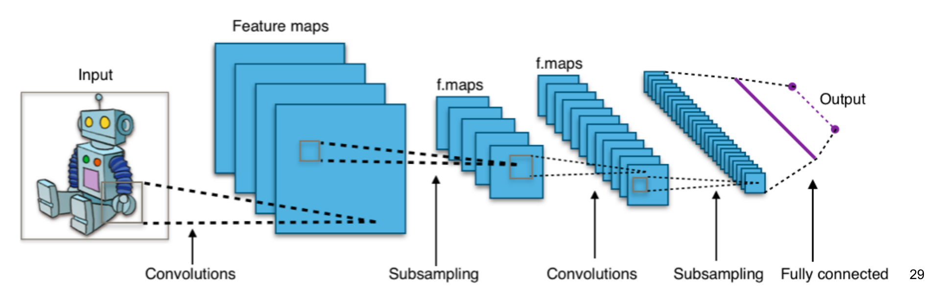
Convolution captures spatial pattern. Pooling (sometimes called subsampling) is the second move: take each 2×2 neighborhood in a feature map and keep only the strongest activation, discarding the rest. This shrinks the tensor by 4× and makes the representation more tolerant to small shifts in the input. It also lets the next convolution see a wider effective receptive field: a 5×5 filter after one pooling step effectively covers a 10×10 region of the original image. After two or three rounds of convolve-then-pool, the spatial dimensions are small enough that you can flatten the result into a vector and feed it into a couple of plain fully-connected layers that do the final classification.
The code is longer but no harder to read:
## mnist2.py (excerpt)

def conv2d(x, W):
  return tf.nn.conv2d(x, W, strides=[1, 1, 1, 1], padding='SAME')

def max_pool_2x2(x):
  return tf.nn.max_pool(x, ksize=[1, 2, 2, 1], strides=[1, 2, 2, 1],
                        padding='SAME')

# Convolutional layer #1: 32 filters, 5x5 each
W_conv1 = weight_variable([5, 5, 1, 32])
b_conv1 = bias_variable([32])
x_image = tf.reshape(x, [-1, 28, 28, 1])
h_conv1 = tf.nn.relu(conv2d(x_image, W_conv1) + b_conv1)
h_pool1 = max_pool_2x2(h_conv1)

# Convolutional layer #2: 64 filters, 5x5 each
W_conv2 = weight_variable([5, 5, 32, 64])
b_conv2 = bias_variable([64])
h_conv2 = tf.nn.relu(conv2d(h_pool1, W_conv2) + b_conv2)
h_pool2 = max_pool_2x2(h_conv2)

# Fully connected layer: 1024 neurons
W_fc1 = weight_variable([7 * 7 * 64, 1024])
b_fc1 = bias_variable([1024])
h_pool2_flat = tf.reshape(h_pool2, [-1, 7 * 7 * 64])
h_fc1 = tf.nn.relu(tf.matmul(h_pool2_flat, W_fc1) + b_fc1)

# Readout layer (10 classes)
W_fc2 = weight_variable([1024, 10])
b_fc2 = bias_variable([10])
y_conv = tf.matmul(h_fc1, W_fc2) + b_fc2
The non-linearity between layers is tf.nn.relu, the rectified linear unit, which is just max(0, x). ReLU is shockingly effective: it is cheap to compute, its gradient is either 0 or 1, and it doesn’t suffer from the vanishing-gradient problem that killed sigmoid networks. When the community switched to ReLU around 2012, networks suddenly trained several times faster than they had with the sigmoids and tanhs that came before.
Re-train, with the Adam optimizer and 1,000 steps:
test accuracy 0.9725
97% after one-tenth as many steps as the linear model. With 10,000 steps (about 18 epochs), the stream looked like this:
step 0, training accuracy 0.15
step 1000, training accuracy 0.96
step 2000, training accuracy 1
step 3000, training accuracy 1
step 4000, training accuracy 1
step 5000, training accuracy 0.99
step 6000, training accuracy 1
step 7000, training accuracy 1
step 8000, training accuracy 1
step 9000, training accuracy 1
test accuracy 0.9898
Compare that to the bouncing 0.85-to-0.95 stream from the linear model and you can see, in the shape of the numbers alone, that something fundamentally different is happening. The model is not gradually scraping its way toward a ceiling. By step 2000 it has already pinned the training batches to 100% accuracy and is mostly refining its general grasp from there. This is the visual signature of a network that has the structural capacity to fit the task. It is also the visual warning sign of overfitting, which we will fix in a moment.
100,000 steps, about 180 epochs:
test accuracy 0.9922
By this point the training run was taking close to fifteen minutes on the V100. That felt like an eternity at the time, and it is comically short by modern standards. People train frontier LLMs for weeks or months, and production CV models for many days. The interval between “submit job” and “see result” shapes the entire rhythm of how you do ML work, and learning that rhythm (knowing when you can iterate freely versus when you have committed to a multi-day run) is most of what separates the experienced ML engineer from a beginner. The dial labeled “patience required” gets a workout that the textbooks rarely mention.
To make the before-and-after plain: with the linear model from earlier in the post (one matrix multiply from pixels to ten class scores, no hidden layers), training accuracy bounced around in the high 80s and low 90s, and test accuracy stalled near 92%. No amount of additional training, no fancier optimizer, no learning-rate tuning could push that ceiling higher. With two convolutional layers feeding into a fully-connected layer (a miniature of the AlexNet recipe), training accuracy locked at 100% by step 2,000 and test accuracy crossed 99%. Same training set, same loss function, same optimizer, same hardware. The only thing that changed was the architecture, the way information flows through the network. That single change is what moved the ceiling, and it is the same lesson AlexNet taught the field in 2012, visible here in miniature.
Now we have an actual deep learning model. Hidden layers between input and output, learned feature detectors that the gradient discovers on its own, real architectural structure. The linear baseline back at the start of the post was the warm-up. Everything from here on is what life is like once you have the real thing.
Knob four: dropout
99.22% is good. It is good enough that you start worrying about a different problem: overfitting. The training accuracy was 100% well before the test accuracy peaked. The network had begun to memorize the training set, not just the underlying pattern.
The 2014 trick for this was dropout: during training, randomly zero out half the activations in a given layer on every step. The network can no longer rely on any specific neuron being available, so it learns redundant representations that generalize better. At inference time, you turn dropout off; the redundancy stays, the network is now more robust.
keep_prob = tf.placeholder(tf.float32)
h_fc1_drop = tf.nn.dropout(h_fc1, keep_prob)
y_conv = tf.matmul(h_fc1_drop, W_fc2) + b_fc2
With dropout added, our MNIST solution gets to 99.35%. The improvement is small because we weren’t overfitting much. The dataset is too easy. Dropout’s effect grows with model size and dataset complexity. Today most modern architectures use it in some form, often alongside batch normalization and weight decay, all of which are different cuts at the same problem of “stop the network from memorizing.” Collectively, these techniques are called regularization.
The cat wall
So I had a working digit classifier. The state of the art on MNIST, in 2017, was less than half a percentage point ahead of what I had trained in a few hundred lines of code on a rented GPU. Time, surely, to do cats.
I sat with this for a while and realized that I had no idea how to do cats.
The MNIST recipe doesn’t generalize, and the reasons why are the most useful thing I learned. Digits are 28×28 grayscale. Cats are full-resolution color photographs of arbitrary aspect ratio, with cats at arbitrary scale, pose, and position. Digits are a closed-world ten-class problem with a clean labeled training set already prepared and waiting. Cats live in a world where the closest dataset to what I wanted was the ImageNet “domestic cat” subset, and even that had been curated by someone with an opinion about what counts. A cat detector also needs piles of negative examples (pictures of everything that isn’t a cat, drawn from a messy heterogeneous world) so the network can learn what “cat” isn’t. MNIST’s negative class for each digit is just the other nine digits; for cats, the negative set is open-ended.
The architectural step from “two-layer CNN” to “production-quality image classifier” is also enormous. The networks that worked on real images had names: AlexNet, VGG, Inception, ResNet. ResNet introduced skip connections specifically to make very deep networks (50, 100, 150 layers) trainable at all. None of this was discoverable from my initial MNIST exploration. The MNIST CNN gave me the vocabulary but not the depth. Once I realized how far the state-of-the-art had moved past my MNIST baseline, my study guide pivoted: there was more leverage in learning what the field had already figured out (which architectures had won, which techniques mattered, how to apply the pretrained checkpoints) than in going deeper on the internals of loss functions and optimizers I had just built from scratch.
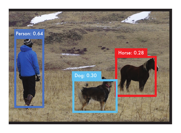
And even with all of that figured out, I’d only be solving classification: “a cat is in this image, somewhere.” What I actually wanted was detection: a tight bounding box around where the cat is. Joe Redmon’s YOLO paper in 2015 was the moment object detection became fast enough to run on live video on commodity hardware. I would later spend time working alongside Joe at a startup that built CV inference for edge devices, which was pretty cool.
What the journey actually taught
Looking back, the most useful thing the project did was teach me, viscerally, what I now think of as the four real facts about training:
1. Training is not just a recipe, it is also a search. The model starts as random numbers. Every step, the gradient pushes the random numbers toward less-bad numbers. The training run is the path through parameter space that this push describes. When researchers talk about “training instability” or “exploding gradients” or “the model didn’t converge,” they are talking about the geometry of that search. Knowing that the search exists, that it’s a real object with a shape, changes how you read every fine-tuning report.
2. The biggest knob is the neural architecture. Optimizers, learning rates, batch sizes, regularization. These are second-order. The thing that decides whether you can reach 99% on your task is whether the network has the structural capacity to represent the function you want. Most “we tried hyperparameter sweeps and didn’t move the metric” stories are stories about hitting the architectural ceiling and not realizing it.
3. Much of the work is data. The cat project stalled, immediately and decisively, on data. There was no clean MNIST-style file waiting for me. Real cat detection meant either scraping the internet (slow, full of garbage labels) or paying Mechanical Turk workers to label images one at a time (expensive and out of scope for a side project). The actual ratio of effort on a from-scratch ML project is something like 70% data work, 20% training infrastructure, 10% model code. Foundation models have changed this somewhat by absorbing the data cost into pre-training, but for any task that requires fine-tuning, the ratio is largely the same. The reason a fine-tune often “doesn’t work” is almost always a data problem dressed up as a training problem.
4. A training loop produces a model; verification gets you the right one. The optimizer is genuinely good at minimizing whatever loss you wrote down. Point it at the wrong loss (wrong objective, wrong proxy, wrong training distribution) and it will faithfully produce a model that minimizes the wrong thing. This is the verification problem at the bottom of the ML stack: a training loop is a faithful executor of whatever you point it at.
You probably don’t need to do this
It would be cruel to end without saying the obvious thing, which is that in 2026 you almost certainly should not train an image classifier from scratch. ResNet-50, EfficientNet, MobileNet, the various vision transformers, are sitting on Hugging Face with permissive licenses, pre-trained on large-scale data, ready to be fine-tuned on your specific task in an hour. The amount of compute that went into producing those weights is on the order of thousands of GPU-days. You are not going to outperform them with a from-scratch run on a single instance.
The same is true, more emphatically, for text. Nobody is training a frontier-grade LLM in a weekend project. The whole point of foundation models is that the heavy training has been amortized. Your job, downstream, is to specialize the existing weights to your domain, evaluate carefully, and deploy.
So why bother understanding what’s underneath?
Because the underneath does not go away. When your fine-tune doesn’t converge, the question is which knob you turn, and the answer depends on whether you understand whether you’re fighting an architectural ceiling, a data problem, an optimizer problem, or a loss-function problem. When your model gives confident wrong answers, the question is whether the training data taught it to be confident about exactly that wrong answer, and that requires being able to think about what the loss was actually rewarding. In 2026, you choose between adapters, full fine-tuning, instruction tuning, RLHF variants, or just better prompting. You are choosing between different ways of moving a known set of weights through parameter space. Knowing the shape of that space helps.
What this is, and what it isn’t
This post is partly a time capsule, the kind of artifact I would have wanted to read in 2017 if anyone had written it at the time. Some of what I have walked through is concept-level scaffolding I had to internalize the hard way, and writing it down for myself was half the reason this article exists.
A small caveat before you close the tab. Even if you fully understand every line of Python in the code above, this is just a description of a simple neural architecture. There is a tremendous amount of system between “Python code describing a network” and “system that actually trains and serves it well at scale,” and almost none of it is in the four hundred lines I walked you through. For example, I said that backpropagation was just the application of the chain rule, but of course there is a bit more to it than that.
That said, what I built in 2017, scaled up, is essentially part of what kicked off the deep learning revolution. AlexNet was structurally a much larger relative of the network I trained on MNIST. Many of the pieces were the same: ReLU activations, dropout, convolutions stacked with pooling. The differences were scale and a few refinements: five convolutional layers instead of two, far more filters per layer, overlapping pooling instead of plain 2×2, heavy data augmentation, and roughly twenty times the parameters, all trained on a much harder dataset. 60,000 grayscale digits became 1.2 million labeled color photographs. An evening of training on my V100 became roughly a week of training on a pair of consumer-grade gaming GPUs (a pair of NVIDIA GTX 580s, the strongest cards Krizhevsky could get his hands on in 2012).
The conceptual leap that made AlexNet historic, that a deep convolutional network trained end-to-end on enough data could blow past every classical method that had been hand-crafted over decades, is exactly the leap visible in the small case I have just walked through.
The big idea was the same. It just got bigger.
References:
- Krizhevsky, A., Sutskever, I., Hinton, G. (2012). ImageNet Classification with Deep Convolutional Neural Networks. The AlexNet paper. The point at which CNNs became the default for image classification.
- LeCun, Y., Bengio, Y., Hinton, G. (2015). Deep Learning. Nature. The canonical overview from three of the field’s founders.
- The Royal Swedish Academy of Sciences. (2024). The Nobel Prize in Physics 2024. Awarded to Hopfield and Hinton for foundational discoveries that enabled machine learning with artificial neural networks.
- Redmon, J., Divvala, S., Girshick, R., Farhadi, A. (2016). You Only Look Once: Unified, Real-Time Object Detection. The YOLO paper. The breakthrough that made real-time object detection (bounding boxes, on video) practical.
- He, K., et al. (2015). Deep Residual Learning for Image Recognition. ResNet. The skip-connection trick that made very deep networks trainable.
- Srivastava, N., et al. (2014). Dropout: A Simple Way to Prevent Neural Networks from Overfitting. The original dropout paper.
- Kingma, D., Ba, J. (2014). Adam: A Method for Stochastic Optimization. The Adam optimizer paper.
- Nielsen, M. Neural Networks and Deep Learning. The clearest free book on what backpropagation is actually doing.
- 3Blue1Brown. Neural networks playlist. If you want the gradient-descent visualization burned into your retinas, watch these.
- Zatloukal, P. (2026). The Bitter Lesson of Agentic Coding. My companion essay on spec-driven workflows and the verification-first methodology for autonomous coding loops.